The two curses of dimensionality
The curse of dimensionality made its print appearance in Richard Bellman’s 1957 book Dynamic programming. It was an outcry over the impossibilities of dealing with functions of many variables when a computer with a million bytes of memory seemed beyond imagination. The expression is uttered only in the preface, but evading the curse motivates the techniques in the book.
Four years later Bellman elaborates on the curse in a short section of his Adaptive control processes. He explains the combinatorial explosion in memory requirements arising when we try to define a function by specifying its values on a grid. The simple example of a one bit function that takes as input one byte requires defining 256 bits, one bit for every possible input. A function of two variables, each a byte, would require $256^2$ bits be specified; for $D$ bytes, $256^D$ bits. Already for $D>20$ we have no hope ever of having that much computer storage (it would require a computer about the size of the Death Star in Star Wars).
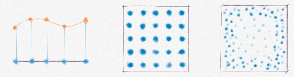
Bellman’s combinatorial explosion would be the extent of the curse if we kept to discrete functions, but a subtle interplay between geometry and combinatorial growth happens when we try to approximate continuous functions. The basic problem can be understood by thinking about well behaved functions of the unit interval $[0, 1].$ One way of approximating any such function is to specify its value on a grid of points.
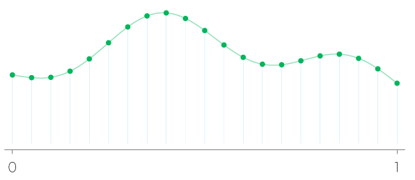
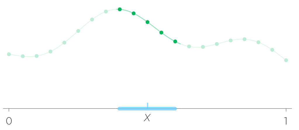
We approximate the value of the function at a point $x$ by centering an interval, say of length $0.05$ around $x,$ and taking the average of all the grid values that fall in that interval as the function’s value at $x.$
There is nothing special about the 0.05, it is the resolution we have chosen as an example. This may be a simplistic algorithm, but all others function approximation algorithms are just elaborations of this idea: Splines? Instead of averaging we fit a curve through neighboring points. Polynomial approximation? The grid is first converted to coefficients. All these algorithms, including our simple one, gather a finite amount of information from nearby points and use that to compute the value at $x.$ The crucial point is that the uncountable infinity of continuous functions is being tamed by the existence of a notion of “nearby”.
If our algorithm demanded that we average five points in an interval of $0.05,$ that would correspond to a grid of points spread every 0.01, or 101 points in the unit interval. When we look at this problem in higher dimensions, Bellman’s combinatorial curse prevent us from having refined grids. The limitation becomes the total number of points we can collect or handle. If we reverse the question and ask how small can the interval be when we have only $M$ points and require 5 in every interval, we get $5/M$ as the grid spacing. If the points are not on a uniform grid, but randomly placed, the interval would have to be even bigger.
Before going to $D$ dimensions, let’s try a similar calculation in two. We pick a point $u$ anywhere on the unit square $[0,1] \times [0, 1]$ and ask for the smallest radius disk that still contains at least 5 of the $M$ points we are given. Each point has to cover $1/M$ of the area, so we need to enclose an area of at least 5 times that, $5/M = \pi r^2$ or
The calculation in $D$ dimensions is similar. Each point has to cover $1/M$ of the $D$-dimensional volume. Instead of asking for 5 points we can be more general and demand $k$ points. The equation we need to solve is
The volume of the sphere in $D$ dimensions is expressed in terms of the Gamma function $\Gamma,$ a generalization of the factorial. If $D$ is even, solving the equation gives that
and when $D$ is odd, $\Gamma(1+D/2)$ replaces $(D/2)!.$
The two fractions in that expression reflect the two curses of dimensionality. The term within parenthesis is the term noted by Bellman in 1957. If we had asked what is the size of a cube that will have $k$ points within it when the space has $M$ points spread uniformly throughout, the answer would have been $r^D = k/M.$ The term with the factorial is the geometrical term not emphasized by Bellman. It grows factorially with the dimension $D:$
| D | factor |
|---|---|
| 2 | 0.318 |
| 3 | 0.239 |
| 5 | 0.190 |
| 10 | 0.392 |
| 15 | 2.622 |
| 30 | 4.6 × 10⁴ |
| 100 | 4.2 × 1039 |
| 300 | 1.5 × 10188 |
| 1000 | 3.2 × 10885 |
That is not a typo: ten to the power 885. And dimensions even bigger than 1000 are common in many vector representations used in machine learning. As the dimensions grow, $M$ will never be large enough to compensate for the geometrical factor.
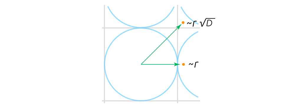
The calculation may be a bit silly, and some may suggest, a mistake, for using a sphere as a neighborhood instead of a cube. After all, both are bounded regions around the image point $u$ where the function is being estimated. But we cannot use the cube and keep a symmetric notion of proximity. The distance between the two furthest point inside the $D$-dimensional cube of side $a$ is $a \sqrt{D},$ the extent of its longest diagonal. The distance between the centers of two neighboring $D$-dimensional cubes is the smaller $a.$ The cube neighborhood and the Euclidean distance cannot both be a notion of similarity at the same time: they are not consistent.
Today, the two aspects of the curse of dimensionality are well known, but if one looks at older articles, Bellman’s combinatorial sense was the only usage I found from 1957 to 1975, the year when Jerome Friedman and collaborators published “An Algorithm for Finding Nearest Neighbors” where they discussed the geometrical factor in the context of the curse of dimensionality. In later papers Friedman and his many collaborators kept emphasizing how high-dimensional spaces are mainly empty and the implications of that vastness in using samples. By 1994 the curse of dimensionality had made it to the title of one of Friedman’s better cited papers.