When collecting data for analysis strange things happen that make their way into the dataset. Sometimes those strange things are mistakes and we try to get rid of them, other times, they really are part of the data and we have to deal with them. Physicists trying to accurately measure the gravitational constant stumble on such strange things: the air conditioner in the lab next door cycles on-and-off creating small temperature variations, or they discover that the variation of the Earth’s rotation rate matters. The knowledge in physics is organized under the assumption that the strength of gravity is a constant, so these effects on the measurements of the constant are considered mistakes. Data analysis should either remove them or, better, correct for them.

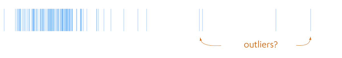
There is another class of strange. In the case of the physicists, there was a theory that molded expectations of how the measurements should behave. In general there is no first-principles theory. In those cases we resort to stochastic models. The model could be as simple as I expect the data to be distributed according to a normal distribution to more complicated things, as it has the same statistics as that simulation I wrote. Given the model (which is a thing that assigns a probability to an event), it may assign very low probability to some of the data points. The data analyst then faces the dillema of what to do with those outliers.

Detecting outliers is a classification problem: we have implicitly assumed that the events we are observing fall into two classes, typical and rare. A very readable introduction to this perspective is offered by Hodge and Austin in their article A survey of outlier detection methodologies published in the Artificial Intelligence Review.

One the most basic classifications schemes is Grubbs’ test (his paper from 1950 incorporates calculations done on the ENIAC). Assume that the data $X_i \sim {\cal N}$ is distributed according to a normal distribution. First studentize the data

Here, $\bar{X}$ is the average of the data and $\mathrm{std}(X)$ is the corrected sample standard deviation (the one with $n-1$ downstairs).

The test asks what happens if we choose a cut point $G_\alpha$ and label outliers all points where $|G_i| > G_{\alpha}$. If all the $X_i$ came from a Normal distribution, for some samples of size $n$ Grubbs’ rule would make a mistake by classifying those points as not from a Normal. To keep these mistakes infrequent, imagine (like a frequentist) that we have many samples of $n$ points. We pick $G_\alpha$ so that only a fraction $\alpha$ of those samples have incorrectly labeled outliers.

If we pick $\alpha$ to be 0.05 (the five percent beloved in the literature), then Grubbs provides a table for what $G_ \alpha$ should be, or we can compute it ourselves using a formula involving the Student $t$ distribution (it is in the Mathematica notebook, which can be downloaded). For example, if there are many different data sets $S_k$ with 15 samples each, then 5% of those data sets $S_k$ will have at least one point $G_i > 2.409$. Whenever there is a Student $t$ distribution involved I’m always suffering trying to figure out if it one sided or two sided. In this case, because of the absolute value in the definition, it is two sided, that is, the outlier could have been 2.409 standard deviations above or below the average.

Grubbs’ test can be generalized to the case where we have a mixture of points, some from a known distribution and a few from an unknown one. The only difficulty is doing the equivalent of the Student $t$ distribution. If you only have twenty or so data points, then it may require some analytical work, but if you have 100 plus, a simple sub-sampling procedure may be all you need.